10 Stats Concepts Every Data Scientist Must Master

When I first dipped my toes into data science, I thought it was all about coding and algorithms.

I was wrong.

Sure, Python and machine learning libraries are powerful tools, but without statistics?

You're trying to build a skyscraper without a foundation.

Let me tell you a quick story.

Back in college, I took a stats class because someone told me it would "probably help someday." I didn't know it then, but that class turned out to be one of the most important steps in my journey to becoming a data scientist.

Here's the thing—data science is really just storytelling with numbers.

And statistics? That's the language we use to make sense of the story.

So, if you're looking to master data science, buckle up. I'm about to cover 10 stats concepts you can't afford to ignore.

1. Population vs. Sample

Imagine you're studying college students in the U.S.

Are you going to survey all of them?

Of course not.

Instead, you grab a smaller group—a sample—and hope it represents the whole population.

Data science works the same way. You rarely get data on an entire population, so you rely on samples. But if your sample is biased or too small? Good luck trusting your results.

Lesson: Always know whether you're working with a population or a sample, and make sure your sample isn't a mess.

...

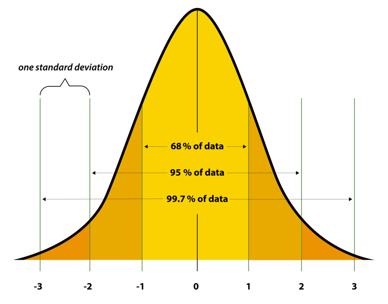
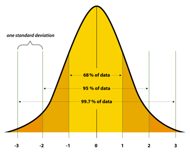
2. Normal Distribution

Ever heard of the bell curve?

That's a normal distribution—where most data clusters around the average, and outliers taper off on both sides.

Why does it matter?

Because many natural processes (height, test scores, errors) follow this pattern. If your data doesn't? You need to stop and figure out why.

Fun fact: Thanks to something called the Central Limit Theorem (more on that later), even weird datasets often act normal if you sample them enough.

3. Mean, Median, and Mode

Think of these as the holy trinity of stats:

• Mean – The average. Add up the numbers and divide.

• Median – The middle value when sorted.

• Mode – The number that pops up most often.

Quick tip: When your data has extreme outliers (like a billionaire in a salary survey), the median is your best friend. It ignores the crazy values.

...

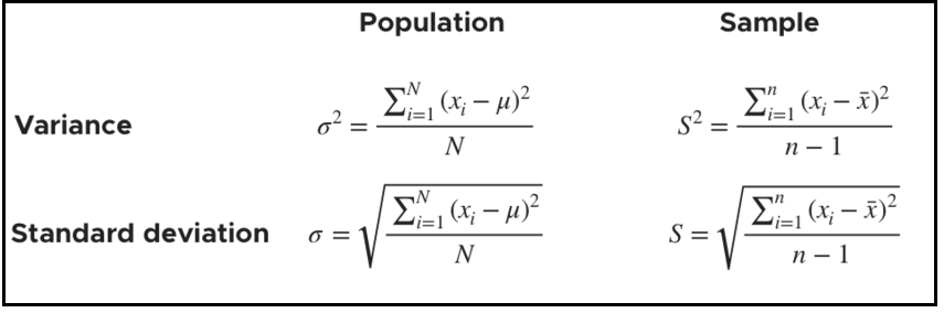
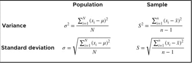
4. Variance and Standard Deviation

Ever been told, "Don't sweat the small stuff"?

Variance and standard deviation measure how much your data "sweats"—or how spread out it is.

• Variance is the average of the squared differences from the mean.

• Standard Deviation is just the square root of variance.

High variance? Your data is all over the place.

Low variance? It's tightly packed.

And if you don't know the difference? Your predictions might miss the mark.

...

5. Covariance and Correlation

Have you ever noticed that when ice cream sales go up, so do shark attacks?

That's correlation—two things moving together.

But does ice cream cause shark attacks?

Nope. They just happen to rise together because more people swim in summer.

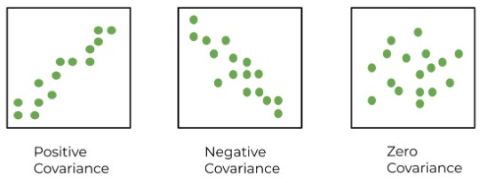
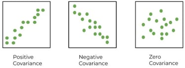
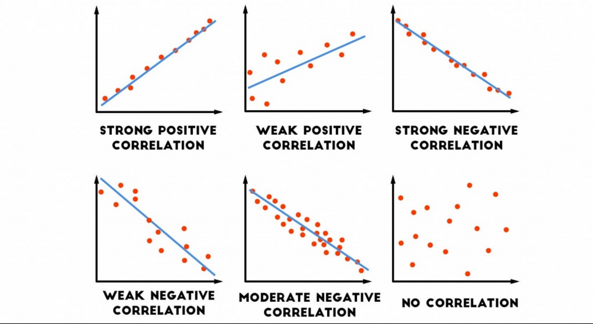
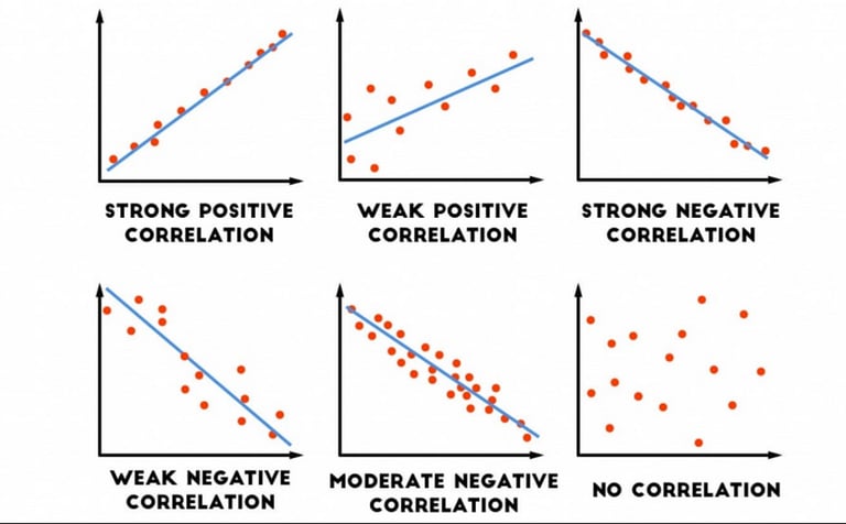
Covariance measures whether two variables move in the same direction. If both variables increase or decrease together, the covariance is positive. If one increases while the other decreases, it's negative.

Think of covariance like watching people at the beach. When the temperature rises, more people buy ice cream and more people swim. Ice cream and shark attacks both rise, but one doesn't cause the other. They're just reacting to the same factor—the heat.

The problem? Covariance doesn't tell you how strong the relationship is.

That's where correlation comes in.

Correlation standardizes the relationship to a scale between -1 and 1, making it easier to interpret:

• 1 means a perfect positive relationship.

• -1 means a perfect negative relationship.

• 0 means no relationship.

Lesson: Covariance shows direction, while correlation shows strength. And always remember—correlation does not equal causation. Dig deeper before jumping to conclusions.

...

6. Central Limit Theorem (CLT)

Imagine you want to know the average height of people in your country.

You can't measure everyone, so you take samples.

Here's the magic: As you take more and more samples, the averages start forming a normal distribution—even if the original data was a mess.

This is why normal distributions are everywhere in stats and machine learning.

It's like a cheat code for working with incomplete data.

...

7. P-Values

You're running an experiment, and you need to know: Is this result real? Or just random luck?

Enter the p-value.

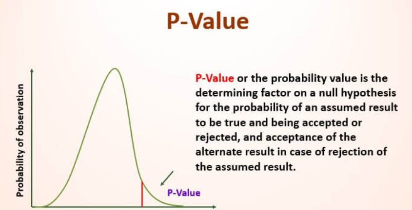
A p-value tells you how likely it is to see your result purely by chance.

• p < 0.05? Statistically significant. You're probably onto something.

• p > 0.05? Don't pop the champagne yet—your result might be random.

Moral of the story: Never trust results without checking the p-value.

8. Expected Value of random variables

Expected value is just the weighted average of possible outcomes.

The expected value is calculated differently for discrete and continuous random variables.

For discrete random variables, mathematically it's calculated as:

E(X) = Σ [ x * p(x) ]

Where:

P(x) is the probability of outcome x

x is the value of that outcome

For example, if you flip a coin and win $10 for heads and lose $5 for tails, your expected value is:

E(X) = (0.5 * $10) + (0.5 * -$5) = $5 - $2.50 = $2.50

This means you expect to win $2.50 per flip on average.

In data science, it's used to predict outcomes and make decisions under uncertainty.

For instance:

• Risk assessment: Calculating the expected loss in insurance claims.

• Investment decisions: Evaluating the potential return of different investment options.

• A/B testing: Estimating the expected improvement from a new feature or design.

• Machine learning: In decision trees and reinforcement learning to choose optimal actions.

Expected value helps quantify the average outcome in scenarios with multiple possibilities, allowing for more informed decision-making in uncertain situations.

...

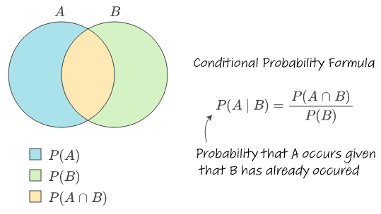
9. Conditional Probability

Imagine you're playing cards.

The chance of drawing a queen changes once you've already drawn an ace.

That's conditional probability—the likelihood of one event, given that another has already happened.

It's the backbone of machine learning models like Naive Bayes, which predict outcomes based on prior knowledge.

Mathematically, conditional probability is expressed as:

P(A|B) = P(A and B) / P(B)

Where:

• P(A|B) is the probability of event A occurring, given that B has occurred

• P(A and B) is the probability of both A and B occurring

• P(B) is the probability of event B occurring

For example, in a standard deck of 52 cards:

• The probability of drawing a queen is 4/52 = 1/13

• But if you've already drawn an ace, the probability of drawing a queen becomes 4/51

Conditional probability is crucial in understanding dependencies between events and making predictions in complex systems. It allows us to refine our probability estimates as we gather more information, making it a powerful tool in data-driven decision making.

...

10. Bayes' Theorem

This one's so important it has its own branch of statistics.

Bayes' Theorem lets you update probabilities as new evidence comes in.

Picture this:

You're testing for a rare disease. A positive test doesn't guarantee you have it—because false positives exist.

Bayes' Theorem calculates the true probability based on prior data.

It's the reason spam filters and recommendation systems work.

Mathematically, Bayes' Theorem is expressed as:

P(A|B) = [P(B|A) * P(A)] / P(B)

Where:

• P(A|B) is the posterior probability: the probability of A given B has occurred

• P(B|A) is the likelihood: the probability of B given A

• P(A) is the prior probability of A

• P(B) is the probability of B

Example: Disease Testing

Let's say a disease affects 1% of the population. A test is 95% accurate (both for positive and negative results).

If you test positive, what's the probability you actually have the disease?

Given:

• P(D) = 0.01 (probability of having the disease)

• P(+|D) = 0.95 (probability of positive test given disease)

• P(+|not D) = 0.05 (probability of positive test given no disease)

Using Bayes' Theorem:

P(D|+) = [P(+|D) * P(D)] / [P(+|D) * P(D) + P(+|not D) * P(not D)]

= (0.95 * (0.01) / (0.95 * 0.01 + 0.05 * 0.99)

≈ 0.16 or 16%

So despite testing positive, there's only a 16% chance you actually have the disease!

Bayes' Theorem is fundamental in probabilistic reasoning and decision-making under uncertainty. It allows us to combine prior knowledge with new evidence, making it invaluable in fields ranging from medicine to artificial intelligence.

...

Final Thoughts

Statistics isn't just math.

It's a survival kit.

Without it, you're guessing. With it, you're solving problems, making predictions, and building machine learning models that actually work.

So if you're serious about data science, don't skip the stats.

It's the difference between looking at data and understanding it.

And trust me—understanding data? That's where the magic happens.

Cheers,

Jake

...

...